Pairs Quant Model
Preface
Duke Energy and NextEra Energy are two of the largest utility companies in the US and both trade on the New York Stock Exchange. The industry has become much more volatile with increased regulations and pressure for these companies to decarbonize and achieve net-zero emissions. The regulatory environment is changing faster than it ever has and large capital expenditures are required of these companies to adjust. This is evident in the recent movements in share prices of industry players such as Duke and NextEra.
A few Key points:
- Operate in the same industry.
- Susceptible to the same economic and market factors.
- Relationship between price movements has increased since 2020.
- Potentially cointegrated.
The above discussion points to a pairs trading strategy that takes advantage of mean reversion tactics. Throughout this document, the full process of a quantitative pairs trading model is explored in detail. Each section is meant to concisely flow through from the rationale of the model all the way to the discovery and findings after testing it.
Rationale
Pairs trading operates under the assumption that two asset prices are cointegrated through time. This means that the mean and variance are considered to be ‘time-invariant’. Above is a depiction of prices through time. I wanted to try this on something that didn’t appear to be perfect at first glance. This means that while one price may move more due to differentiating factors, there is a chance the spread will mean revert.
Cointegration
Cointegration is a concept that won Clive W.J. Granger a nobel prize in 2003, and is an excellent measure for pairs trading. This measure allows the construction of a single stationary time series from two asset price time series. This is done by finding the cointegration coefficient, or the cointegration beta.
This differs from correlation in that correlation describes the relationship between the returns, whilst cointegration is a long-term relationship between prices.
- Returns are normally used for analysis because they are regarded as being much closer to stationary.
- Spurious correlation is the result of a regression on unrelated prices, as prices are generally non-stationary.
- In order to find out if the linear regression on prices produces a stationary residual, the Augmented Dickey-Fuller test can be applied to two assets that appear related.
- If the residual is stationary, this indicates that the two asset prices are cointegrated.
- Returns will be used to calculate the hedge ratio.
The problem becomes which asset to select as the dependent variable. To solve this, run the regression twice and select the dependent variable that produces the highest significance in the ADF test. Below is an output of results from the ADF test on NEE - DUK:
| Test.Statistic | Critical.Value |
|---|---|
| -2.601 | -2.57 |
Spread 1, which utilizes NEE as the dependent variable, has a more negative test statistic which is significant at the 90% confidence level. This isn’t fantastic, but it means we can assume our series is somewhat stationary and use this spread to conduct our quantitative trading strategy, utilizing a beta of 0.625 (calculated by a regression on returns) on DUK as our hedge ratio.
Signals & Rules
To set trade signals, I’ll be using Z-score. The Z score measures how many standard deviations the spread is from the mean. For this strategy, I will use a 10 day window for mean and standard deviation.
- When the Z score crosses the upper threshold (parameter 1), Sell NEE and buy DUK (Short the spread).
- When the Z score crosses the lower threshold (parameter 2), Buy NEE and Sell DUK (Long the spread).
- When the profit-take and stop-loss thresholds (parameter 3 and 4) are crossed, it is time to exit.
- Stop-loss will remain at -2.5 and 2.5.
- Profit take will remain at -0.2 and 0.2.
Below is a chart depicting the process from a one year snipped of the data for clarity. The short and long parameter values chosen are arbitrarily set and will be optimized later.
The logic of the model will be built so as to accommodate for all of the factors shown above, and execute positions exactly according to the signals and rules laid out.
Here is a plot of what the strategy looks like with the set values in the plot above, over the same time frame:
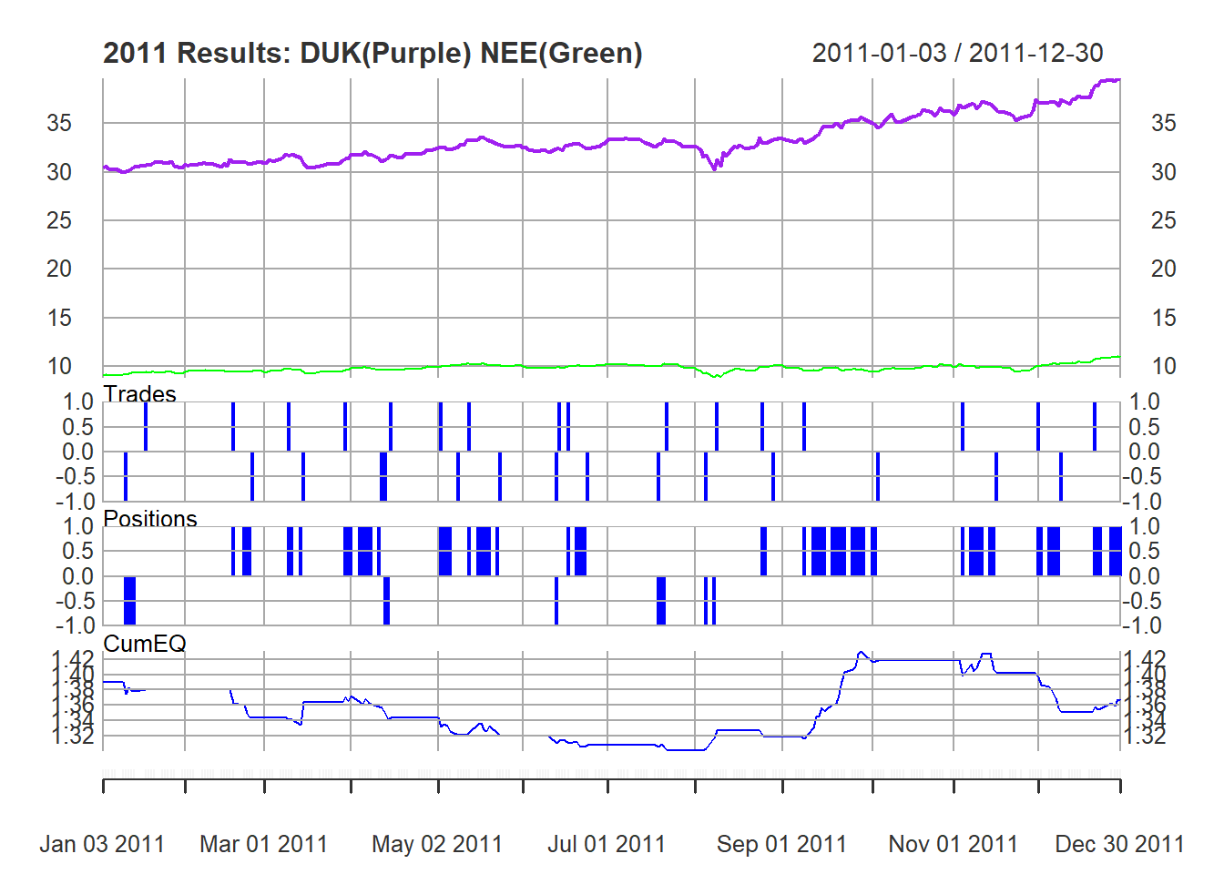
The data used to observe the strategy (training data) is from January 2000 to the end of 2019.
Risk Appetite and Desired Exposure
I am attempting to make this model as usable and realistic as possible for me. As this is my first construction of a pairs model and I have very limited capital to deploy, I have baked in the following constraints in the trade execution logic:
- I only want to hold one position at a time. This means even if the z-score moves across an execution parameter before moving across the profit-take line, no new trades will be entered. This is to minimize my exposure and limit the transaction costs associated with a very high volume of trades. This constraint will help, but the nature of setting up a model like this by using the variation in z - score will still result in a fairly active model producing a high number of trades.
- Stop-Loss and Profit-Take levels have been included. These constraints act to minimize risk. Stop-Loss is included so if the spread continues to move to extreme deviation I’ll cut my losses. As I am using adjusted closing prices to compute the z-score, Profit-Take levels will minimize the risk in a large movement at the open the following day, or if the z-score approaches zero but does not cross, I’ll still realize profit. These were actively included in the execution logic as well.
Optimizing In Allignment With Risk Appetite
During optimization, I will look to optimize the z-score values for entering into a long or short position on the spread that will maximize my cumulative return. This will be combined with minimizing the drawdowns of my strategy due to the limited capital I have available to deploy and avoid large losses. I also want to compare the percentage of winning periods to cumulative return to test for any over fitting. The exact thresholds (while maximizing Cumulative Return) are as follows:
- Drawdowns less than 30%.
- % win greater than 30%.
After running iterations over different parameter values, the below charts show the optimal parameter values that maximize the value added based on my defined risk appetite indicators.
A couple thoughts based on the above plots:
- Drawdowns have very little variation. I believe this is due to me incorporating profit-take and stop-loss levels into the model, which combats against large hits to capital preservation.
- % Win higher than anticipated.
- All objectives seem to peak in a similar area.
Strategy Results and Backtesting
After reviewing the data shown in the plots, the following parameter combinations hit the mark:
| par1 | par2 | CumReturn | Ret.Ann | %.Win | DD.Max |
|---|---|---|---|---|---|
| 0.6 | -2.0 | 3.73 | 0.08 | 0.52 | -0.28 |
| 0.6 | -2.1 | 3.70 | 0.08 | 0.52 | -0.26 |
| 0.5 | -2.1 | 3.34 | 0.08 | 0.52 | -0.27 |
The model wants the short trigger to happen sooner (Z = 0.6) and the long trigger slightly later (z = -2.0). Lets backtest this from 2020 onwards. The price movements since 2020 look very favorable for a strategy of this nature:
The performance of the position on the backtesting data:
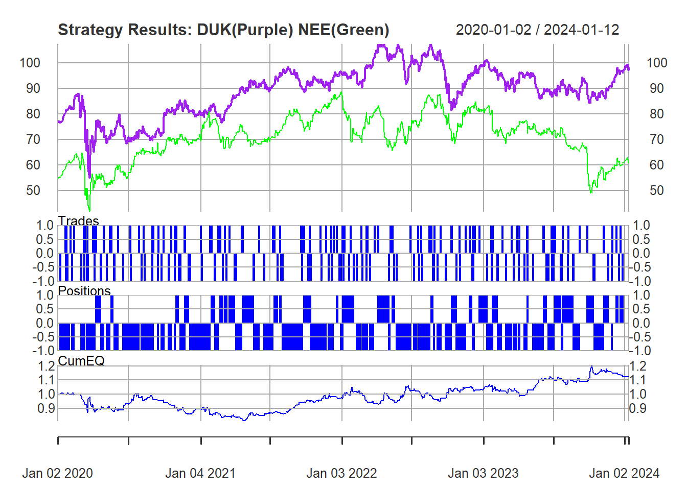
Before looking further, lets look at transaction costs on the NYSE. 98 spread trades (196 total) were executed at a cost per transaction of $0.0012. This assumes only entering 1 spread position per transaction at a volume of 1, which I described in my risk appetite above. This is immaterial with such a low volume but if position size were to be scaled up, this could get significant.
Lets Check the stats:
| Metric | Value |
|---|---|
| CumReturn | 0.12 |
| Ret.Ann | 0.03 |
| %.Win | 0.50 |
| DD.Max | -0.20 |
This is compared to a Buy and Hold Return (DUK + NEE) of 29%. The returns of the pairs strategy is 14%, which is significantly lower. The 50% win indicates over fitting is not a risk here, as the model only kicked out 14% cumulative equity. This is a quality return, but I was hoping to out pace the buy and hold.
Learnings and Review
I tried to take on something that would be challenging and stretch my abilities. I wanted to conduct a strategy on two assets to increase the complexity of building the model, setting out the parameters, and building in the required logic to pull it off. This not only tested my trading knowledge, but also really pushed the boundaries of my coding ability. Below is a list of either concerns I have, things I learned, or assumptions I had to make simply because I could not effectively include them.
- The hardest part was building a strategy function that actually worked with my parameters, as well as the profit-take and stop-loss levels that I wanted to include.
- This model, while yet only holding one position at a time, has a very high frequency of trades. Even though I briefly discussed this, I would of liked to find a working way to include transaction costs in the model itself.
- There are a lot of short positions. These are made under the assumption short selling is always possible, and liquidity is high enough. Finding a way to account for this would greatly improve the model.
- I tried to use stop-loss and profit-take to add complexity in place of ‘scaling in and out’. With the frequency of trades already occurring, scaling up my position would require a lot more complexity and analysis. I based this on holding one spread unit so I could focus more on having an accurate base.
- I am assuming cointegration throughout the entire time series. Ideally, I’d rather test for it over small windows and include that in my trade logic.
- I am happy that I was able to produce trade signals that opened and closed positions to my specifications.
- The ADF test did not produce great results. I still carried out the model, but this would be great to test on a pair that I find with a better fit.
- I initially used the price beta as my hedge ratio, which resulted in a much higher level of cumulative returns. After making this adjustment and correctly using the beta found when regressing on returns, the strategy performance was less optimal, but the process is now correct, barring my logic is 100% correct when calculating returns.
This was an excellent exercise. I am happy with how much it taught me about pairs trading, quantitative modelling and learning how to actually implement and test a strategy in practice.